What is the relationship between maximizing loudness, psychoacoustics and perceptual lossy compression?
In the world of audio engineering, you often hear the folk-wise adage, “If it sounds good, it is good.” This is often a response to overly technical or esoteric commentary on techniques or technologies employed. But, if hearing is ultimately subjective, what does it mean to “sound good?” A minimum requirement of a satisfactory mix is that all the intended sounds can be heard on a reasonable playback system.
The field of psychoacoustics is concerned with how humans’ ears and nervous systems perceive sound rather than the strictly measurable properties of sound and recorded audio itself. Psychoacoustics also help us understand why many sticky technical points that mix engineers get caught up on don’t matter outside the world of precision measurement, because most if not all people can’t hear them.
Whether we realize it or not, today’s consumer music experience is deeply influenced by the convergence of psychoacoustic and computer science research. Most people today listen to music via streaming services that utilize “lossy” compression technology that is possible thanks to decades of research on auditory masking phenomena applied to perceptual data compression. In a nutshell, lossy compression attempts to identify the parts of an audio signal that the average user won’t be able to perceive well, and stores those sounds with significantly less information or no information at all, while prioritizing the parts that the user does perceive in higher resolution.
At its core, audio data compression is quite straightforward. Software removes redundant information and approximates the audio signal over a discrete time period to compress a piece of digital audio data. The approximation becomes less accurate the longer the sample time-period. Because of this, an MP3 with a high sampling rate (short sample durations) has a greater quality than one with a low sampling rate. However, file formats like mp3 are simply standards for compatibility on playback. The encoding process varies by implementation, and there are sophisticated approaches to dividing the source signal into 32 frequency bands and analyzing each to maximize the perceived quality of the output stream based on psychoacoustic principles of temporal and frequency masking.
As it turns out, as engineers tuned and perfected this approach to perceptual compression over the course of a decade, with the first practical implementation of mp3 specification in 1992 they were able to remove 90% of the original signal information while still representing the sound in subjectively “transparent quality” (depending on encoder settings). In other words, human hearing is so imperfect that up to 90% of the raw information in the data for music could be removed, or, more accurately, “simplified,” without the average user noticing a significant difference on average consumer equipment in double blind (ABX) tests.
If we consider that massive potential margin of irrelevance due to psychoacoustic principles that make a 128kbs mp3 music file sound “good enough,” understanding those principles can be invaluable for mix engineers to grasp how many complex attributes in a mix coexist and to identify common pitfalls and frustrations in practice.
The details of psychoacoustics and especially auditory masking are highly technical, so let’s attempt to distill them down to their essential practical principles.
1. Frequency Masking
Signals in the same or nearby frequency range have a tendency to “mask” or block each other. Two instruments playing at the same volume in the same frequency range make it challenging to distinguish the details of either individual part. Lower frequency content has a wider masking effect. As we move up the harmonic spectrum the masking effect is narrower. Human hearing is optimized to hear midrange, coincidentally the frequencies associated with human speech, and thus can better distinguish competing frequencies.
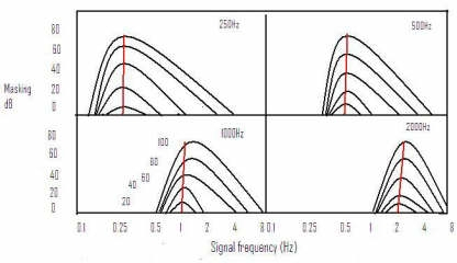
2. Masked Threshold
A masking frequency raises the minimum level at which a competing frequency can be heard and distinguished. This is common sense. If a guitar with distortion is playing a big chord at a loud volume, the level at which a person singing can be heard is increased.
3. Critical Bandwidth and Auditory Filters
This is important in terms of tones being too close together in frequency bandwidth to distinguish or one tone masking an equivalent or nearby tone of lower volume. The critical bandwidth of a masker frequency applies to curve around it, meaning a well designed codec can take advantage of that phenomenon and reduce the resolution of masked frequencies, or simplify them. The equal widths of the subbands do not accurately reflect the frequency dependent behavior of human hearing. The width of a “critical band” as a function of frequency is a good indicator of this behavior. Many psychoacoustic effects are consistent with a critical band frequency scaling. For example, both the perceived loudness of a signal and its audibility in the presence of a masking signal is different for signals within one critical band than for signals that extend over more than one critical band.
4. Temporal (time based) Masking
A transient signal, like a loud snare drum will diminish the perceived loudness of sounds both before (pre-masking) and after the transient (post-masking), which I assume is not to say that we can hear something before it happens, but that our cumulative perception of that sound is modulated after the fact. This becomes important when we consider the impact of heavy limiting on mixes to achieve perceived loudness.
5. Equal Loudness Contour & Absolute Hearing Threshold
We hear different frequencies unequally. Lower frequencies and very high frequencies are harder to hear. This is why the “loudness” button and “smiley face” eq sounds good, especially on lower quality systems. Many smaller systems today automatically apply a significant loudness contour eq curve. Mixes that sound natural should not be flat, but should have a pronounced increase in low frequency energy. Vinyl records had difficulty storing powerful low frequency energy without the stylus skipping, or “jumping out of the groove” and thus had to be compensated for with a standard RIAA equalization curve. Modern digital formats don’t have this limitation and over the past twenty years the average bass response of popular music has substantially increased.
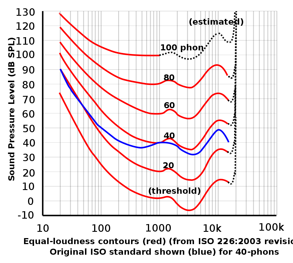
The Absolute Threshold of Hearing (ATH) is the level at which a person can hear a sound 50% of the time. Sensitivity varies from person to person, changes as we age and follows the similar pattern of the equal loudness contour shown above.
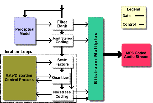
At a simplified level, the mp3 and similar lossy codecs perform the following functions
- Perform a 1024-sample fast-fourier transform (FFT) on each half of a frame (1152 samples) of the input signal, selecting the lower of the two masking thresholds to use for that subband.
- Each frequency bin is mapped to its corresponding critical band.
- Calculate a tonality index, a measure of whether a signal is more tone-like or noise-like.
- Use a defined spreading function to calculate the masking effect of the signal on neighboring critical bands.
- Calculate the final masking threshold for each subband, using the tonality index, the output of the spreading function, and the absolute threshold of hearing (ATH).
- Calculate the signal-to-mask ratio for each subband, and passes information on to the quantizer.
For all the gory technical details of how this works, Hydrogenaud.io wiki provides an excellent overview. But the takeaway is that the codec implementations do attempt to analyze and take advantage of temporal and frequency masking in order to remove stuff from the signal as transparently as possible.
All mixes involving more than one sound source have some degree of masking. Hundreds of video tutorials and articles are available on the internet that discuss techniques to identify and compensate for them. Various software products are available that assist in this process. The most straightforward approach is carefully listening for areas where two sound sources are competing in the same frequency and adjust them with some combination of dynamic level (sidechain compression) or complimentary equalization. This article won’t rehash those techniques, but instead will focus on the implications of the perceptually “irrelevant” information in popular audio and how loudness maximization and lossy consumer formats impact it.
I clearly recall the dawn of the widespread adoption of mp3 in the late 90s. Like most people, I was on a poor quality “dial-up” connection and my first impressions were a combination of amazement, excitement and concern. The average user was well aware of the technical limitations of average consumer computer hardware of the period. Everything back then was far more scarce: bandwidth, cpu cycles, RAM and storage space. The mp3 was a triumph of convenience. As I downloaded my first mp3 files, probably at the then default 128kbps that aspirationally claimed to be “near CD quality,” I immediately noticed that while it certainly wasn’t, it was totally acceptable in comparison to the sound quality of lower quality cassette mix tapes that I had grown up with.
When I heard mp3 compression on songs that I had listened to hundreds of times and was deeply familiar with, I could clearly hear the difference. Songs with simpler arrangements and less density translated well. Dense rock, percussive and orchestral music did not translate well on early implementations of the mp3 codec, even at higher settings. Mp3 rips of an old favorite of mine, My Bloody Valentine’s Loveless were particularly bad at translating frequency masking, and even today I can’t stand to listen to it on lossy formats, even though the implementations of various lossy codecs have markedly improved. That album is widely considered a masterpiece of sonic density. Masking is absolutely everywhere, and my youthful ears that fell in love with that music on compact disc could hear a universe of rich texture and detail in layer upon layer of distortion, modulation and reverberation. It is a good example of program that is simply too complex for lossless algorithms to reliably determine which data is irrelevant.
Other lossy encoded recordings that underwhelmed me were jazz tracks featuring a range of prominent cymbals that have complex and closely spaced transients. Performances by jazz drummers playing complex patterns on ride cymbals and high hats “smeared,” and had strange “ringing” artifacts.
Twenty five years later entire generations of music lovers have grown accustomed to the sound of lossy compression. In fact, a popular anecdotal study in 2009 noted that college students preferred it in blind comparisons because the “sizzle” that the potential artifacts seem to impart.
Not all people hear equally. There’s hearing loss or hearing deficiency, of course, but furthermore, some people are born with or have developed the ability to listen better than others. Martha Harbison notes in a 2013 Popular Science article that many subjects can hear the differences in both temporal and frequency masking. Musicians often have the most skill at differentiating time and frequency differences between tones.
“To test if the human ear was accurate enough to discern certain theoretical limits on audio compression algorithms, physicists Jacob N. Oppenheim and Marcelo O. Magnasco at Rockefeller University in New York City played tones to test subjects. The researchers wanted to see if the subjects could differentiate the timing of the tones and any frequency differences between them. The fundamental basis of the research is that almost all audio compression algorithms, such as the MP3 codec, extrapolate the signal based on a linear prediction model, which was developed long before scientists understood the finer details of how the human auditory system worked. This linear model holds that the timing of a sound and the frequency of that sound have specific cut-off limits: that is, at some point two tones are so close together in frequency or in time that a person should not be able to hear a difference.“
Martha Harbison from “Why Your Music Files Sound Like Crap”
The study concluded that the assumptions of the linear model were not the case. In essence, all of the lossy audio compression algorithms are based on an outdated understanding of how the human ear works. (Perhaps this is technically incorrect, as Ogg Vorbis and Opus do take non-linearities of masking into account, but close enough for click bait).
When dynamic range is sacrificed in a mix in order to be exciting and competitive with the loudness of modern hits that consumers have come to expect, masking is even more challenging and is a good reason to consider adding a loudness-compensated limiter or maximizer on your mix buss to preview the complex implications of that process on the balance of a mix. Hey, there are even mp3 preview plugins.
How Does Loud Mastering Affect Lossless Encoding Quality? Let’s test to find out!
Brickwall limiters and special algorithmic limiters called maximizers can significantly impact the sound of a mix, especially the transients.
- Things that were previously masked, or barely perceived in the background come forward and get louder.
- Transient details that previously “poked out” and gave a track “depth” are often flattened and lost.
- Spatial effects like reverb and echo increase in loudness.
- In ADSR terms, the decay and sustain of all signals is increased, also increasing their relative temporal and frequency masking potential.
- Common examples are snare drums, vocals, keyboards and guitars in the midrange, and bass guitar and kick drum in the low frequency range. These sources are often prominent in dense rock mixes and, depending on the arrangement, may fiercely compete for spectrum.
Heavy limiting for loudness may impact the linear prediction models used in lossy compression in unexpected ways. More of the sound sources are forced into the upper range of loudness, increasing the amount of wideband signal that a codec may deem “important” and thus should be encoded at higher resolution. If the codec’s bitrate target is the same, what then? While I haven’t found any evidence of how this potentially effects subjective sound quality, if lossy algorithms are taking advantage of encoding lower volume and masked frequency information at lower bitrates, what happens when there’s less dynamic range? It seems that increased density, including more competing transient detail would be harder to encode and more prone to artifacts and smearing.
To test this hypothesis, a section of the song, “Havona” by Weather Report was processed through a high quality mastering maximizer and automatically imported back into a DAW session. I chose this song because it has particularly prominent and complex cymbal work. Mp3 “stem” files were then encoded at 128kbps cbr for both the original 16bit 44.1k audio and the 16bit 44.1k maximized audio and imported back into the session and checked for the short gap inherent to LAME encoding (the DAW compensated for it). A null test was printed between the original and its mp3 copy and again for the maximized version. Both resulting mp3 files were exactly the same size, confirming that the encoding was constant.
A null test is a critical test in audio engineering to determine the mathematical difference between two waveforms. An exact copy of an audio file with the polarity inverted will null to zero when combined (summed). The result is absolute silence — in fact, the resulting print will contain no information. The same test across two files pre and post some type of processing will sum to reveal only the differences between them. For purposes of our tests, the waveforms are perfectly time aligned automatically by our DAW.
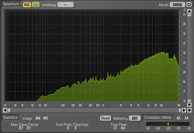
The null test reveals the shocking amount of musical information that is lost or modified in the conversion for both versions. Clearly audible, the original null result immediately reveals a lot of complex transient cymbal details. The frequency analyzer set to “average” the frequency energy across the entire sample shows that the most of the frequency spectrum was affected, with significantly more loss in the high frequency range. Cymbals are particularly problematic, but almost all instruments are audible.
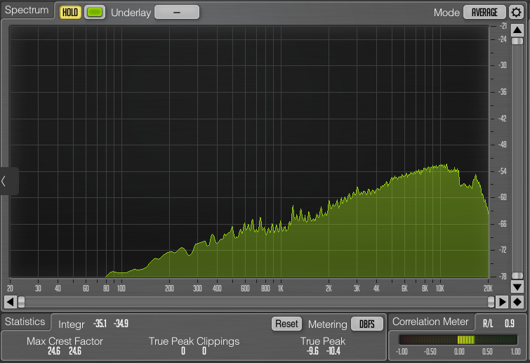
Since the maximized audio has a significantly less dynamic range, it’s no surprise that the result from the analyzer is flatter, but it is worth noting that the maximized version at bottom despite being attenuated while I was running the average (because it was too loud) seemed to have more relative audio loss in the lower frequencies. Visually, both are reasonably comparable in terms of average information loss given the difference in dynamic range. This averaging visual representation normalized the information too much to be useful.
The images of the nulled waveforms reveal some interesting differences in the way that the decay of sound sources are inconsistently more pronounced from section to section of the maximized file vs the original, which is more consistent, possibly due to the sustain and decay. It’s fair to say again that mp3 compression has a very difficult time with transient ringing and smearing of cymbals. Again, this has more to do with the maximizer than the mp3 process.
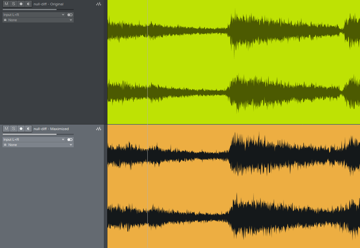
The null difference audio clips tell a more interesting story. The maximized version has more complete audio overall, where the original seems to be more selectively targeting the transients and high frequencies — like a sketched outline of details around the original signals. This tells us that additional harmonic information is being removed from the maximized version by the algorithm as it struggles to distinguish temporal and frequency masking with all frequencies flattened. Or perhaps, the codec is really just linear and we’re obviating a low bitrate rendition of louder midrange.
Unfortunately, without more accurate measurement techniques, these results are not conclusive. There’s no smoking gun, but the audio samples lend support to our hypothesis that heavily limited audio provides less “breathing room” for linear perceptual compression algorithms to subtract audio with a reasonable degree of transparency. Or maybe it’s really just not that sophisticated, and we’re just hearing a louder version of the same junk because the source was louder and “slammed.” The audio examples indicate that heavy limiting has audible impact on the 128kbps LAME 3.100 codec used by Presonus Studio One, and perhaps more importantly, 128kbps is very lossy indeed.
If you’re shocked by how much information is present in the samples above, an artist created an entire rather spooky song out of the “lost information” in the “original” mp3 for Suzanne Vega’s Tom’s Diner.
So what do we do about it in our mixes? If you want to maximize sound quality in all areas, including mobile streaming, mix with more dynamic range!
In 1998, I heard an experienced successful engineer say that, with the ever decreasing headroom of modern mastering, when you can’t go up, you have to go big or wide. In other words, if you technically can’t go louder, you have to compensate by widening the stereo image, changing the overall frequency curve (usually more midrange) or temporal space (length) to simulate size or the acoustic phenomenon of louder sounds overcoming the resistance of air and reflecting back to your ears in a natural environment. If your verse is already at “11“, the only way to make your chorus seem louder is to widen the stereo image, increase relative midrange (because it’s perceived as louder) or add more delay and reverb. That may be the single most important nugget of mix-related wisdom I’ve ever heard.
A very snappy loud snare with a sharp transient attack and little to no source decay may sound great in a dynamic mix, popping out comfortably of the dense midrange and then moving out of the way. Temporal masking will naturally occur, and at loud volumes, the acoustic reflex response of the ears will contract, causing an “organic” sensation of compression. This is what you hear when a live band plays in an acoustic space. Our sense memory of this is why compressed drums sound like “loudness”. But once heavy limiting is applied, that same snare may be overwhelmed and masked by other midrange sources. The snare may be buried in the mix. In that case, where there is no headroom to allow a satisfactory distinguishable transient, more compression, saturation or a spacial effect like a reverb on the isolated snare signal can restore the snare to its perceived forward position, compensating for the absence of natural temporal masking – the less transient snare must made “wider,” “fatter” and “flatter.” The trade-off is that the denser snare now represents a larger and wider frequency masking event, potentially competing with your vocal and guitars for more critical midrange bandwidth.
A dynamic mix that has a nice ratio of transient energy simply sounds different. Adding compression to an entire drum kit demonstrates the opposite effect – everything becomes “fatter” and more exciting, but the incredibly wide dynamic range potential of the kick, snare, toms, cymbals and reflections of the acoustic space then wreaks havoc on the mix balance like a chaos monkey randomly masking everything in the mix, at which point the engineer often resorts to a rube goldberg machine of complex sidechain ducking schemes.
Mix engineers working in pop, pop country, R&B, electronic and rock genres use far more compression on sources than you’d think, and probably far more than they used to when compressors were expensive and a pain in the ass to patch into a board (the popularity of SSL desks changed that by the late 70s by building in a compressor on every channel!). They do this to constrain the potential random interplay of dynamic range and transients of those sources — choosing to strictly control them with volume automation. Depending on the arrangement and sources, aggressive compression on all sources can be a recipe for a fatiguing and lifeless mix, but it reduces the range of variability that may arise from mastering and the wide range of consumer experiences.
Years ago, I had been frequently listening to high quality masters of Tom Petty & The Heartbrakers 1976 eponymous album on my home system and while driving to the store, heard the same song on the radio that I had just been listening to at home. The mix balance of the song sounded completely and utterly different on the radio broadcast due to the heavy limiting and multiband compression. I was hearing parts and instrumentation that I barely noticed on the original master. It sounded almost like a different song entirely.
One of the reasons music of the 70s often had so much dynamic range was the improved quality of emergent audio technology from studio to consumer made it favorable. People were increasingly listening to music at home on better systems — and the immense popularity of wall-to-wall carpet probably improved the acoustics of the average listening space. Usable dynamic range above noise floor in the analog domain was challenging and considered a goal for maximizing fidelity in popular consumer formats. The closest thing to a “competitive loudness space” across titles was radio and jukeboxes, and the former was largely moot, as dynamic range/loudness was normalized automatically. Radio stations applied heavy brickwall limiting to program before transmission for many reasons: FCC regulations, the severe limitations of dynamic range inherent to FM (much less AM technology), to level match song to song, and to make their station louder and exciting than the competition. One could say that radio invented the loudness war long before the labels did.